Multi Head Attention 多头注意力

Multi Head Attention

多头注意力（Transformer 原文章的图）

大多数时候，我们希望模型能够从相同的输入里面学到不同的东西（或者说，能学到不同方面的东西）. 而如果只有一个 Attention 模块，很显然不论怎么学，模型最终只能学习到一个概率分布. 所以为了改进这一点，我们引入 Multi-Head Attention

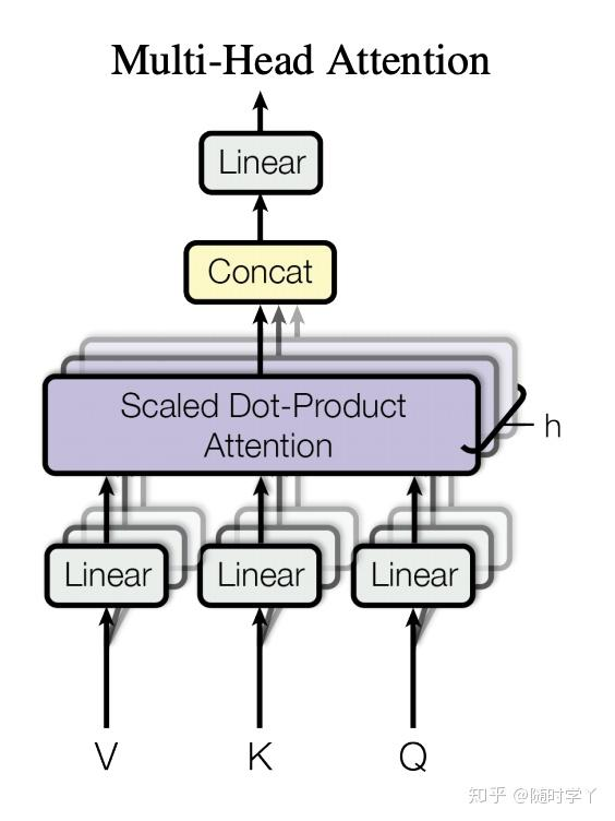
每一个 Attention 的输出称为 Head，所以我们有很多的 Attention Head，假定我们有 $h$ 个 Attention Head. 对于输入的 $\bold{Q,K,V}$ ，我们先用 $h$ 个 Fully Connected Layer 分别 transform $\bold{Q,K,V}$ 得到 $\bold{Q}_i,\bold{K}_i,\bold{V}_i$ . 然后分别输入 $h$ 个 Attention Head. 最后，将这 $h$ 个 Attention Head 的 Output 拼接起来，再最后经过一次 Fully Connected Layer.

用数学语言描述的话就是，令 $\bold{Q}\in \R^{d_q}, \bold{K}\in\R^{d_k},\bold{V}\in\R^{d_v}$ ，单个 Attention Head 的数学描述为

\bold{h}_i=\texttt{Attn}(\bold{W}_i^{(q)}\bold{Q}, \bold{W}_i^{(k)}\bold{K}, \bold{W}_i^{(v)}\bold{V}) \in\R^{p_v}

其中 $p_v$ 为 Attention Head 的输出维度， $\bold{W}_i^{(q)}\in\R^{p_q\times d_q}, \bold{W}_i^{(k)}\in\R^{p_k\times d_k},\bold{W}_i^{(v)}\in\R^{p_v\times d_v}$ . 最后，我们还会接上一个 Fully Connected Layer $\bold{W}_o$

\bold{W}_o\begin{bmatrix} \bold{h}_1\\ \bold{h}_2\\ \vdots\\ \bold{h}_h \end{bmatrix}\in\R^{p_o}

进一步解释

我们的 Multi Head Attention 的流程如下.

首先输入三个三维张量 $\bold{Q,K,V}$ . 此时，这三个张量分别有各自的 batch size $b$ 、包含的 token 数量 $n$ 、token 的 embedding vector 的维度 $d$ （我们这里把 embedding vector 理解为包含其语义信息）.

现在，假设我们的 Attention 模块处理的词向量空间的维度为 hidden dimension $D$ ，并且包含 $h$ 个 Attention Head.

那么很显然，第一步，我们先需要把三个张量的词向量维度都先投影到统一的 Attention Space 里，这样才能让 Query 对应的 $\texttt{K-V}$ 加权和更加 make sense. 即，使用 $3$ 个 $\texttt{nn.Linear}$ .

# LazyLinear 的作用是，自动检测最后一个维度并构造矩阵
# LazyLinear(20)(tensor of size (x, y, z)) => tensor of size (x,y,20)
self.Wq = nn.LazyLinear(D)
self.Wk = nn.LazyLinear(D)
self.Wv = nn.LazyLinear(D)

# ......
# 现在，这三个张量ed最后一维都是 Hidden Dimension (h) 了
Q = self.Wq(Q)
K = self.Wk(K)
V = self.Wv(V)

接着，我们需要让每一个 Head 处理词向量维度的一部分，注意这里是词向量维度而不是 token 数量维度！

我们可以这么理解：我们希望每一个 Attention Head 学习到的是不同 token 之间不同领域的管理。关键点在于不同领域，如果按照 token 数量进行切分，那么实际上变成了每个 Head 学习句子局部之间的关系，这肯定就不对了。所以这一段对应的张量操作，其实是把最后一维 $(D,)$ 进一步拆分成 $(h, \frac{D}{h})$ .

def transpose_qkv(self, x: torch.Tensor):
    x = rearrange(
        x,
        "batch seq (heads eachhead) -> batch seq heads eachhead",
        heads=self.num_heads,
    )
    return x


Q = self.transpose_qkv(Q)
K = self.transpose_qkv(K)
V = self.transpose_qkv(V)

对 $\bold{Q,K,V}$ 都做完 transpose_qkv()，我们接下来就想像 normal Attention 那样：对于每一个 batch，其中对于每一个 head，对 $\bold{Q}$ 的 $n_q$ 个 token 计算 $n_k$ 个 score，然后再对 $\bold{V}$ 求加权和。从张量形状的角度来看，这个变化过程为

(b, \boxed{n_q}, h, \boxed{\frac{D}{h}}) \texttt{ @ } (b, \boxed{n_k}, h, \boxed{\frac{D}{h}}) \implies (b, \boxed{n_q}, h, \boxed{n_k})

这个需求其实和 $\texttt{torch.bmm}:\R^{n\times m\times \ell} \texttt{ @ } \R^{n\times \ell\times p}\mapsto\R^{n\times m\times p}$ 很像. 然而 $\tt torch.bmm()$ 只接受三维的张量. 所以，我们考虑把 $b,h$ 这两个维度压缩到一起（反正他们在过程中是不会变的），然后执行 $\tt torch.bmm()$

这里，注意到把 $b,h$ 两个维度压缩到一起后，其实和 $\tt "batch" \times \#words\times \#dim$ 的形式已经差不多了，所以这里可以直接套用 normal Attention 的实现. 最后再把结果的形状转回去即可.

def tf(self, x: torch.Tensor):
    return rearrange(
        x,
        "batch seq heads eachhead -> (batch heads) seq eachhead",
    )

Q = self.tf(Q)
K = self.tf(K)
V = self.tf(V)

output = self.attention(Q, K, V)

于是乎得到的张量形状是

(bh, n_q, \frac{D}{h})

再用 rearrange 把它变回 $(b,n_q, h\times \frac{D}{h})$ ，最后再套一层线性层 $\texttt W_o$ 即可

output = rearrange(
    output,
    "(batch heads) numq eachhead -> batch numq (heads eachhead)"
)
output = self.Wo(output)

return output